
Fifty Years of Counting Orcas: Southern Resident Demography in Nine Charts
A Julia analysis of NOAA's demographic database on the Southern Resident killer whales: 227 individuals, 1976–2025. Kaplan–Meier curves by sex, age pyramid, fecundity, interbirth intervals and first-year survival — what the numbers show, and what they cannot say.
https://morrisonkuhlsen.com/southern-resident-killer-whales-demography-julia-kaplan-meier/
There is one wild animal population in the world where every individual has a name, a birth year and a family tree. They are the Southern Resident killer whales — the three family groups, called J, K and L pods, that move through the Strait of Georgia, the Salish Sea and the coastal waters of Washington and British Columbia.
Since 1976 they have been photographed and counted one by one, every year. The result is exceptionally rare in ecology: not a sample, not a mark-recapture estimate, but the complete census, with birth and death years for virtually every individual across five decades.
I took that database — published by NOAA in the noaa-nwfsc/srkw-status repository — and analysed it in Julia. This post walks through the nine charts it produced, what each one says, and, at the end, what they honestly cannot say.
1. The database
The orca.csv file has one row per individual, and the essential columns are few:
| Column | What it is |
|---|---|
animal |
individual identifier (J002, L025, K021…) |
birth |
year of birth |
death |
year of death — NA if the animal is alive |
pod |
pod and matriline of origin |
matriline |
matriline (named after the oldest female in the lineage) |
mom |
mother’s identifier, when known |
sexF1M2 |
1 = female, 2 = male, NA = undetermined |
That is 227 individuals, with births recorded from 1910 to 2025: 151 deaths and 76 animals alive. By sex: 105 females, 91 males and 31 of undetermined sex — nearly all of them calves that died before they could be sexed. By pod: J with 66 records, K with 44 and L with 117, spread across 20 matrilines.
Two methodological notes before any chart:
- The analyses start in 1976. The systematic photo-identification census — the technique of recognising each animal by the white patch behind the dorsal fin, the saddle patch, developed by Michael Bigg in the 1970s — only becomes reliable from that point on. Earlier records exist, but they are retrospective reconstructions.
- The temporal resolution is the year, not the day. The database stores birth year and death year. That means “survived its first year” here literally means “did not die in the same calendar year it was born” — which is slightly different from surviving 12 months.
2. Fifty years and no net gain
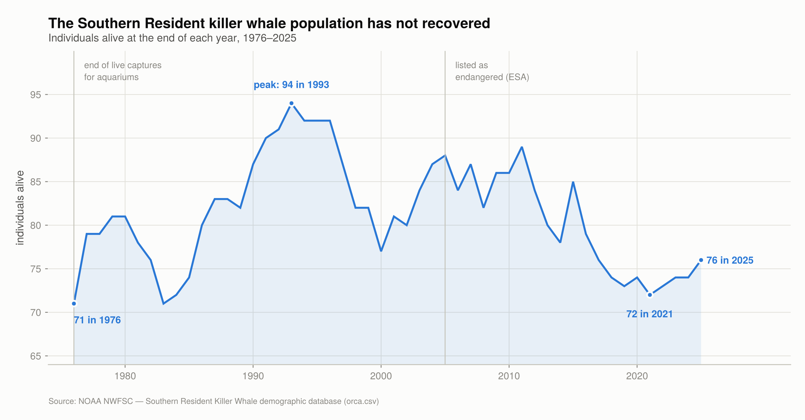
The population had 71 individuals in 1976, climbed to a peak of 94 in 1993, dropped, oscillated, and reached 2025 with 76 — after a recent low of 72 in 2021. That is 19.1% below the peak, and only five animals more than half a century ago.
It is worth splitting the series into two regimes and fitting a log-linear regression to each (the slope of $\log N$ against year estimates the instantaneous growth rate $r$, and $\lambda = e^{r}$ is the annual population multiplier):
| Period | $r$ (per year) | $\lambda$ | Growth | $p$ | $R^2$ |
|---|---|---|---|---|---|
| 1976–1993 | $+0.0111$ | $1.0111$ | $+1.11\%$/yr | $0.00082$ | $0.51$ |
| 1993–2025 | $-0.0064$ | $0.9937$ | $-0.63\%$/yr | $5.4 \times 10^{-8}$ | $0.62$ |
The two periods have opposite signs and both are statistically significant. After live captures ended, the population grew for seventeen years at just over 1% per year. Since 1993 it has been shrinking consistently, at about 0.63% per year, and that trend explains 62% of the variance — this is not noise.
One figure that misleads: the geometric mean $\lambda$ across the whole series is $1.0014$ (standard deviation of the annual $\lambda$ values: $0.0422$). Looked at that way, from 1976 to 2025 growth appears flat-but-positive. It is the average of two opposing regimes, and it describes neither of them.
3. The decline is entirely in L pod
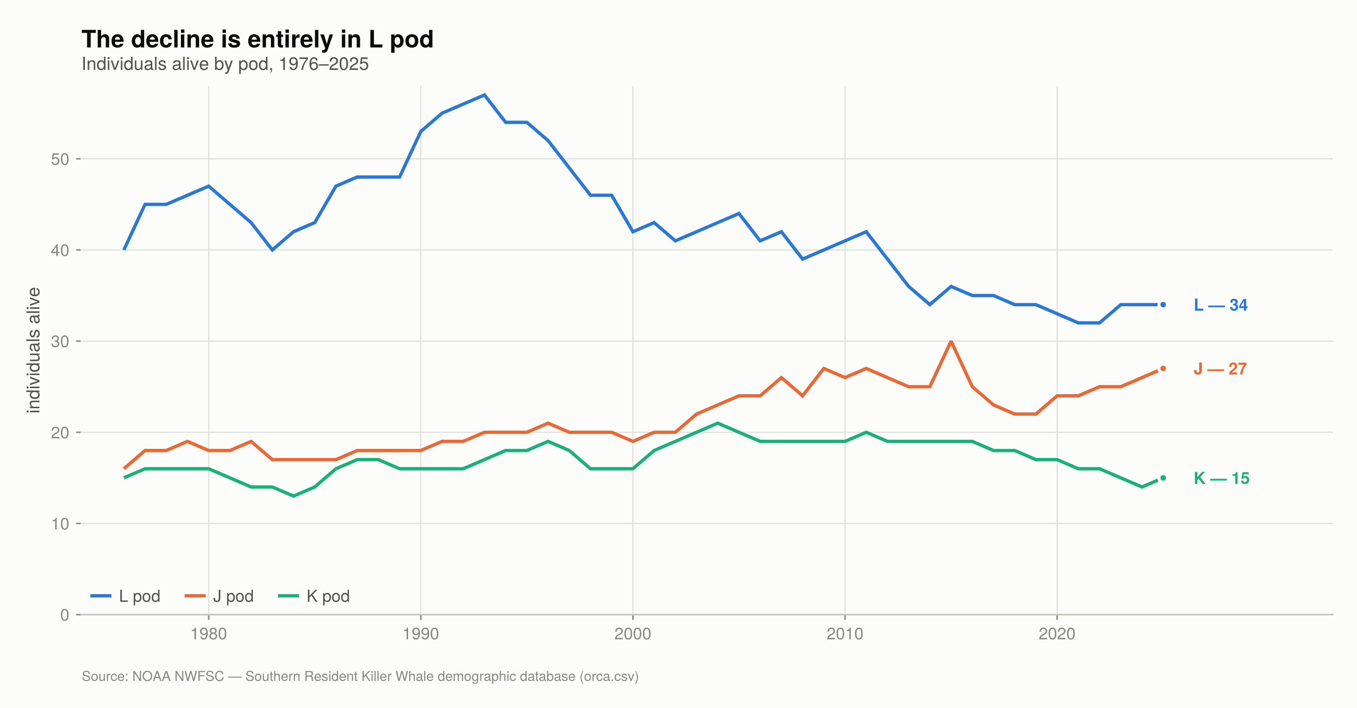
Summing the three pods hides the essential fact:
| Pod | 1976 | Peak | 2025 |
|---|---|---|---|
| J | 16 | 30 | 27 |
| K | 15 | 21 | 15 |
| L | 40 | 57 | 34 |
J pod grew 69% over the period. K is exactly where it started, fifteen animals in 1976 and fifteen in 2025 — after having reached 21. And L, the largest of the three at 40 individuals, lost 15% and sits 23 below its own peak.
The entire net decline since 1993 is concentrated in L pod. That matters because pods are not interchangeable units: they are matrilineal groups with their own vocal dialects and partly distinct foraging ranges. Concentrating the losses in a single pod is not equivalent to spreading them across all three.
4. Births and deaths nearly cancel out
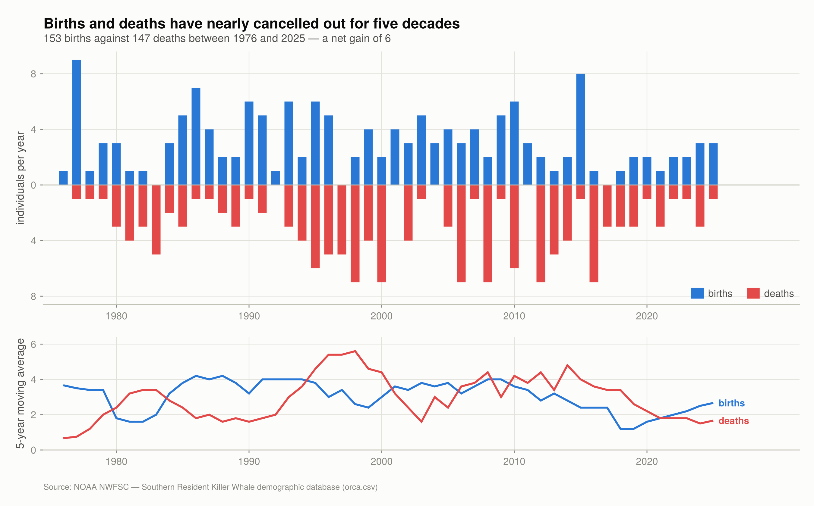
Between 1976 and 2025 there were 153 births (mean 3.06/year) against 147 deaths (2.94/year). Cumulative balance over fifty years: +6 animals.
The linear trend in births is $-0.0213$ per year, with $p = 0.302$ — that is, not significant. The birth series is too noisy for a straight line fitted to fifty annual points to detect anything. This is worth stating plainly: anyone who wants to claim “births are declining” cannot support it with a simple regression.
What does hold up is the balance of the last decade: 1.70 births per year against 2.60 deaths per year. A population losing nearly one animal a year does not recover by accident.
5. The age pyramid: where are the old males?
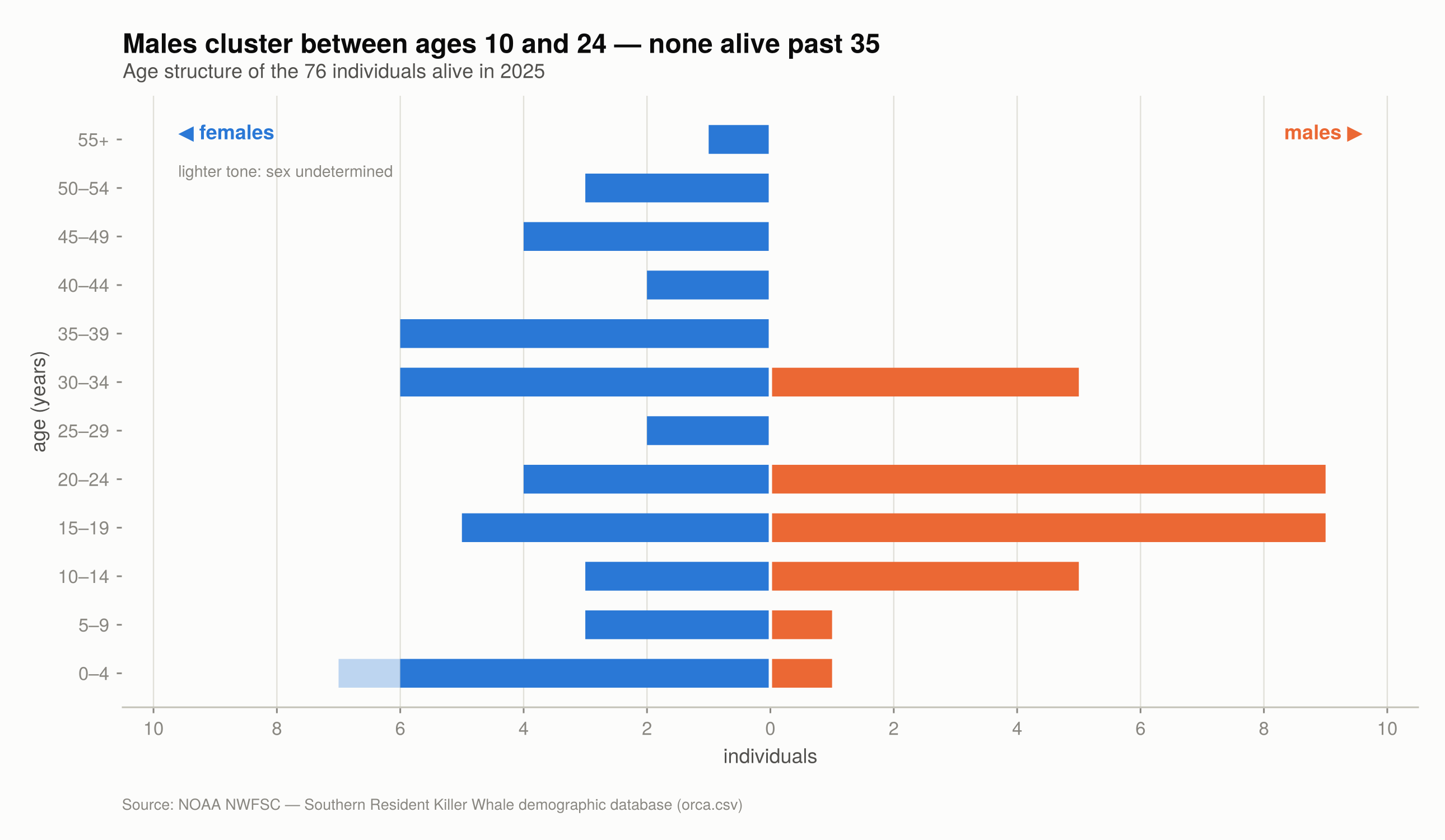
Of the 76 alive: 45 females, 30 males and 1 of undetermined sex.
The chart shows a brutal asymmetry. Living males cluster between 10 and 24 years old, and the oldest is 34. There is no living male above 35. On the female side, eight are past 42, and the oldest in the population — L025, recorded as born in 1928 — is 97 in the database.
This is not a quirk of this population. It is the pattern for Orcinus orca: females live much longer than males, and it is on that asymmetry that the entire literature on cetacean menopause rests (I return to it in section 8).
6. Kaplan–Meier: females survive twice as long
Survival is the kind of question you cannot answer with a mean. Of the 227 animals, 76 are alive — their lifespans are unknown; we only know they are at least the current value. Ignoring them biases everything downward; treating current age as final age biases it too. The correct treatment is right censoring, and the standard estimator is Kaplan–Meier.
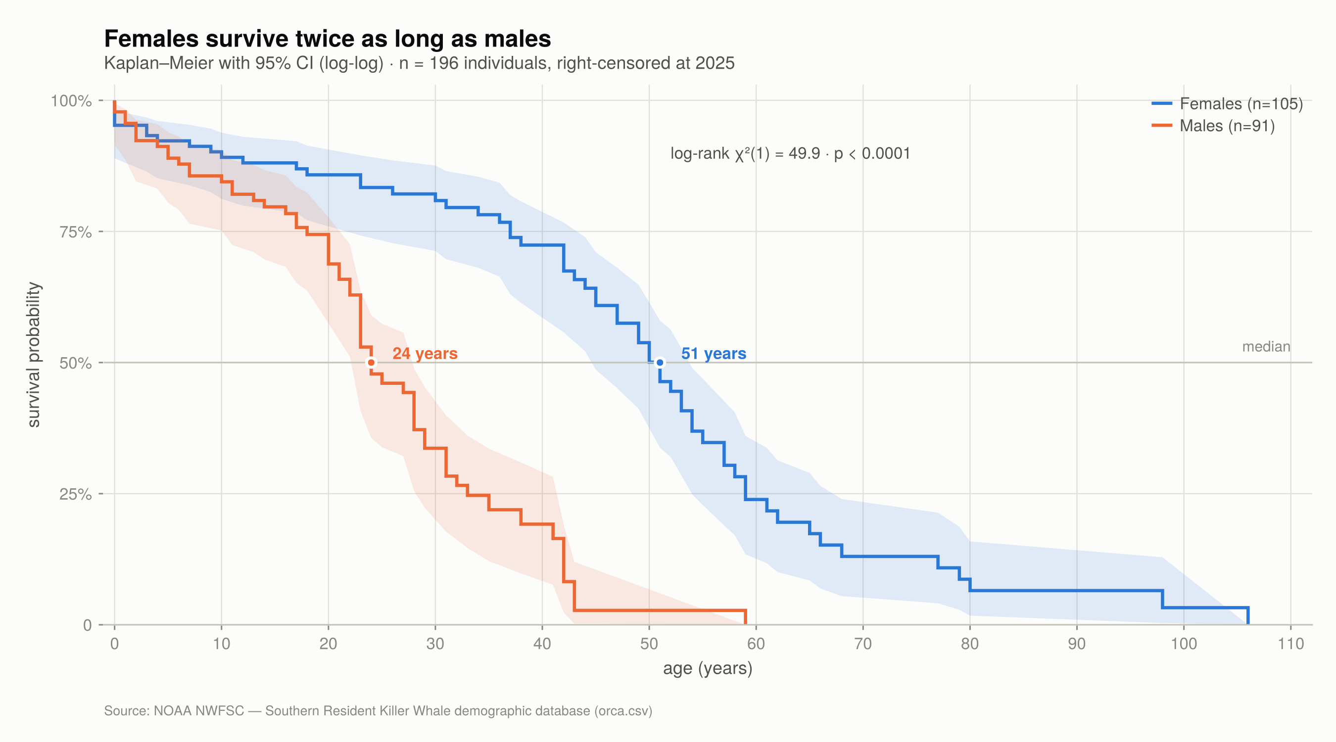
Median survival: 51 years for females, 24 years for males. Log-rank test: $\chi^2(1) = 49.93$, $p < 0.00001$.
A $\chi^2$ of nearly 50 on one degree of freedom is enormous. The confidence bands of the two curves come nowhere near touching around the medians. The difference between the sexes is the most robust finding in this entire analysis.
Note the shape of the curves as well. Both fall quickly in the first years — infant mortality dominates the beginning — after which the female curve flattens into a long plateau while the male curve keeps descending at a steady rate. These are two different mortality regimes, not the same curve shifted.
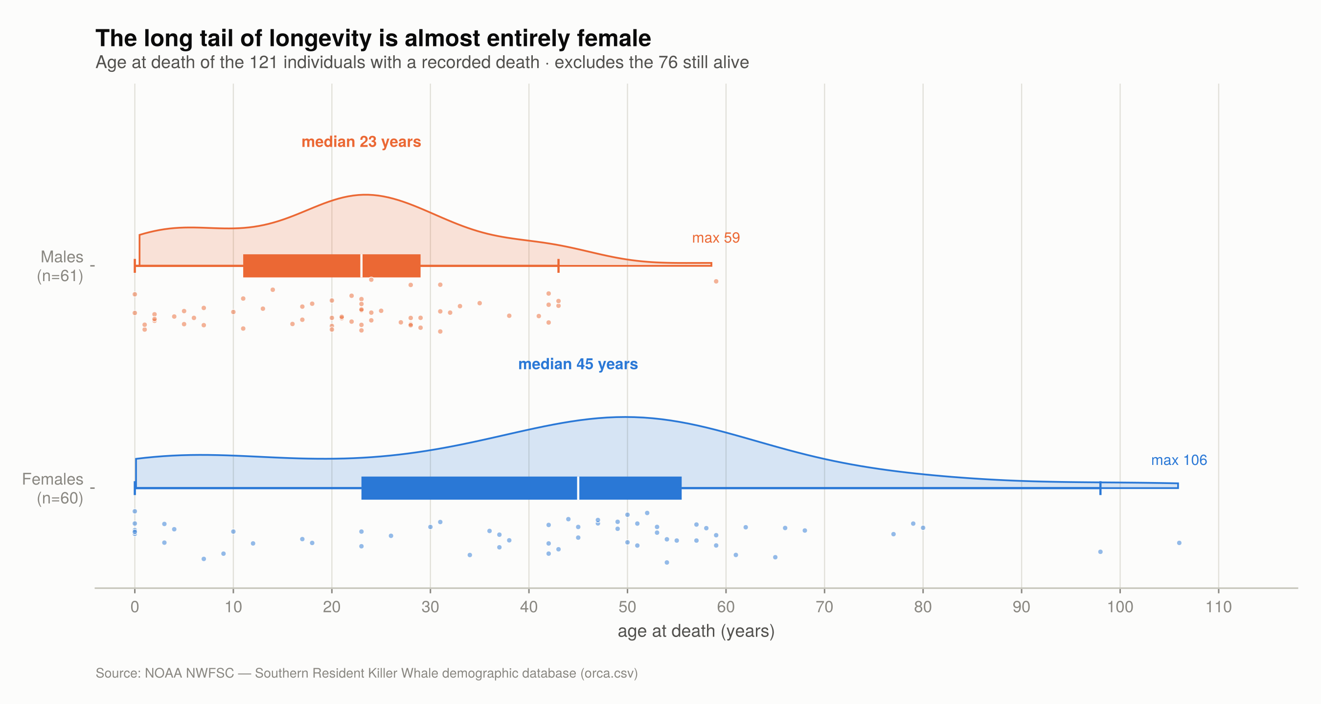
7. The long tail of longevity is almost entirely female
| $n$ | Median | Mean | Maximum | |
|---|---|---|---|---|
| Females | 60 | 45 years | 41.1 | 106 |
| Males | 61 | 23 years | 21.5 | 59 |
The female median is essentially double the male one, consistent with Figure 5. But what jumps out is the asymmetry of the distributions: the male one is compact and ends at 59; the female one has a long tail stretching to 106.
An important caveat, which I will press on in the limitations section: that maximum of 106 years belongs to J002, known as Granny, with a birth year of 1911 in the database. That age is disputed. The original 1911 estimate came from assuming the male J001 was her son; later genetic testing showed he was not, and biochemical analyses suggested a much lower range, somewhere between 60 and 80. The number sits in the database because the database preserves the historical estimate, not because the question is settled.
8. Reproduction: when, and how often
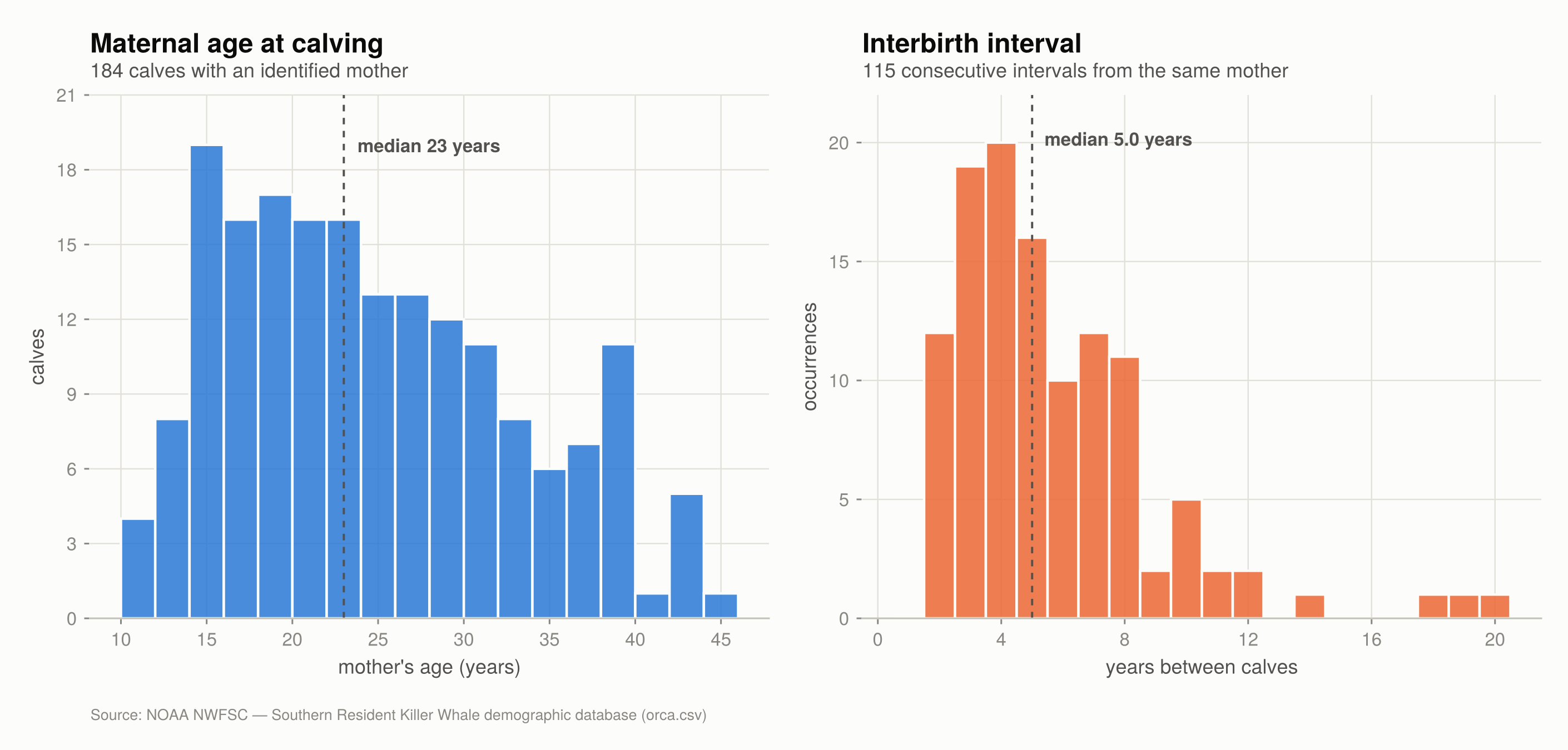
Cross-referencing the mom column against each mother’s birth year gives 184 calves from 69 different mothers:
- Maternal age at calving: median 23 years (mean 24.3; quartiles 17 and 30; observed range 10 to 45).
- Interbirth interval: median 5 years (mean 5.7; quartiles 3 and 7; observed from 2 to 20 years, $n = 115$).
- Calves per mother: median 2, maximum 7.
The upper bound on maternal age — 45 years — is the demographic signature of menopause. Killer whales are one of very few non-human species with a long post-reproductive life: females stop calving around 40 and can live another three or four decades. In this database, eight living females are already past 42.
Why would a female stop reproducing with decades of life ahead? The literature has converged on two complementary explanations, both tested on this very population: old females that reproduce alongside their daughters have calves with far higher mortality — the intergenerational reproductive conflict of Croft et al. (2017) — and post-reproductive grandmothers measurably increase their grandoffspring’s survival, especially in years of low salmon abundance (Nattrass et al., 2019). Stopping calving and switching to care is, on the arithmetic, the higher-return strategy.
The median interval of 5 years between calves, combined with a reproductive window of roughly 30 years, puts the population’s biological ceiling at a very low level. There is no fast-recovery scenario for an animal with this life history — even under ideal conditions, the demographic response takes decades.
9. Fecundity has halved
This is, to me, the most worrying chart of the set.
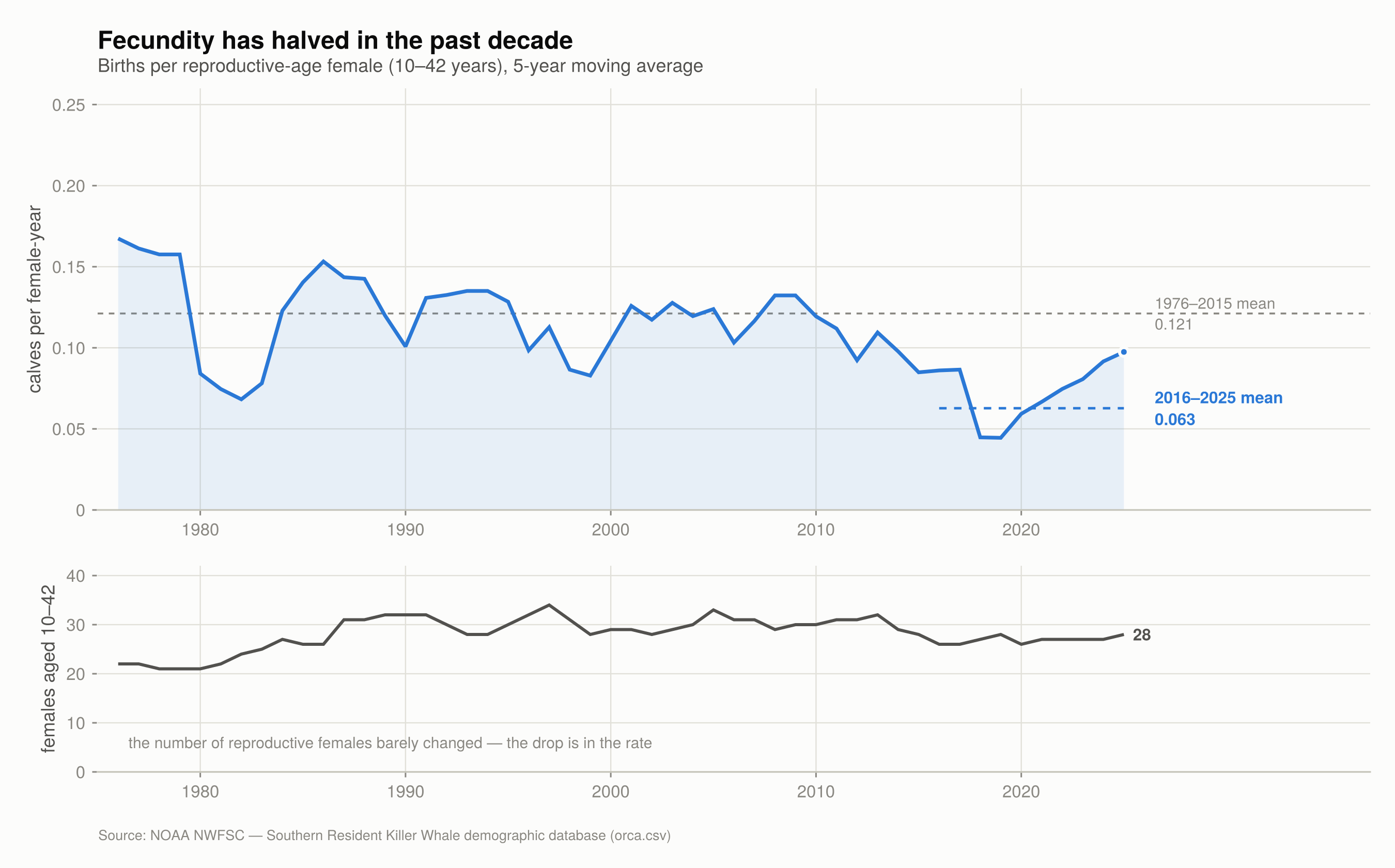
Counting raw births is not enough: with fewer fertile females, fewer calves is the natural outcome. The measure that matters is fecundity — births per reproductive-age female per year.
| Period | Fecundity |
|---|---|
| 1976–2015 | $0.1212$ calves/female-year |
| 2016–2025 | $0.0627$ calves/female-year |
The recent rate is 52% of the historical one. To test whether that could be sampling fluctuation, I took the historical fecundity as a reference rate and asked how many births would be expected over the last decade given the observed number of fertile females year by year. The natural model is Poisson:
17 births observed against 32.2 expected under the historical rate — $p = 0.0050$.
And the lower panel of the figure closes the argument: the number of females aged 10 to 42 was 34 at its peak (1997) and is 28 today. That is an 18% drop, not 50%. The denominator barely moved; what fell was the rate.
This is exactly what the literature predicted. Ward, Holmes and Balcomb (2009) showed that fecundity in these whales tracks the previous year’s abundance of Chinook salmon. Wasser et al. (2017), measuring hormones in faecal samples collected by detection dogs, found up to two-thirds of pregnancies failing between 2007 and 2014, with nutritional-stress markers seven times higher in the females that lost their pregnancies. The drop that shows up here as a number — 0.121 to 0.063 — is, on the biological side, pregnancies that never reach term.
10. First-year survival: no clear signal
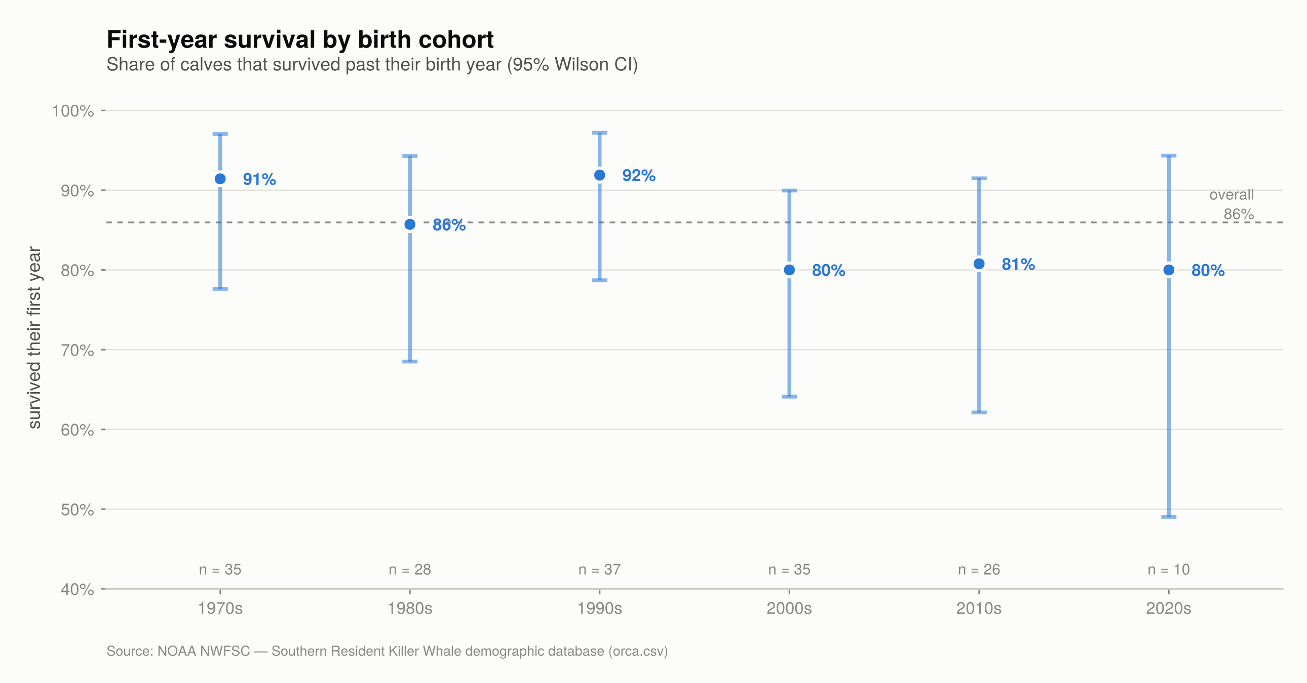
| Cohort | $n$ | Survived | Proportion | 95% CI |
|---|---|---|---|---|
| 1970s | 35 | 32 | 91.4% | [77.6%, 97.0%] |
| 1980s | 28 | 24 | 85.7% | [68.5%, 94.3%] |
| 1990s | 37 | 34 | 91.9% | [78.7%, 97.2%] |
| 2000s | 35 | 28 | 80.0% | [64.1%, 90.0%] |
| 2010s | 26 | 21 | 80.8% | [62.1%, 91.5%] |
| 2020s | 10 | 8 | 80.0% | [49.0%, 94.3%] |
The overall proportion is 86.0% ($n = 171$). There is an apparent drop from the 1970s–1990s cohorts (85–92%) to the 2000s–2020s ones (80%), but the confidence intervals overlap heavily — with thirty-odd calves per decade you cannot distinguish 80% from 92%.
I used the Wilson interval rather than the Wald one precisely for this reason: with small $n$ and $p$ near 1, Wald produces bounds above 100% and poor coverage. Wilson fixes both problems.
The correct reading of this figure is absence of evidence, not evidence of absence. And it contrasts interestingly with Figure 8: the fecundity drop is statistically detectable; a drop in calf survival is not. The apparent bottleneck sits before birth, not after it.
11. What these numbers do not say
An honest analysis needs a list of the things it cannot support.
- Nothing here is causal. There is not a single environmental variable in this database — no salmon, no vessel noise, no PCBs. The causal explanations I cited come from other studies with other designs. What I did here is describe the demography.
- Old ages are estimates, not observations. Animals already adult at the start of the census had their ages back-calculated. J002 (106 years) is the extreme and disputed case, and it single-handedly pulls up the female mean and maximum. Without it, the observed female maximum drops to 59 years.
- Annual resolution compresses the first months. A calf born in November and dead in January counts as having survived its first year; one born in February and dead in December does not. That adds noise to Figure 9 in a direction that is hard to predict.
- Calves that die very early may never enter the database. If a stillbirth or a newborn dies before being photographed, it never becomes a row in the CSV. The fecundity computed here is therefore a floor — and true neonatal mortality is higher than measured.
- 2025 is partial. The database is a snapshot; the official census may still be revised. The value of 76 should be read as provisional.
- 31 individuals have undetermined sex and fall outside the by-sex analyses. Since they are mostly animals that died early, excluding them tends to inflate both Kaplan–Meier curves slightly.
- The 10-to-42 reproductive window is a convention. It comes from the species’ life-history literature, but it is a hard cut applied to a gradual process — shifting it by two years changes the fecundity denominator.
12. Methods
The whole analysis lives in a single Julia script, with CSV.jl and DataFrames.jl for the data and CairoMakie.jl for the figures. The statistical procedures were implemented directly, with no survival-analysis package:
- Log-linear regression by ordinary least squares on $\log N_t$, with standard error, $t$ statistic and $p$-value from Student’s $t$ distribution with $n-2$ degrees of freedom.
- Kaplan–Meier with right censoring at 2025. Confidence intervals built on the $\log(-\log S)$ scale with Greenwood’s variance, which guarantees bounds inside $[0, 1]$ — unlike the naive symmetric interval.
- Two-sample log-rank test, with the statistic $(O_1 - E_1)^2 / V$ compared against a $\chi^2$ with one degree of freedom.
- Wilson interval for the per-cohort survival proportions.
- Two-sided Poisson test for the last decade’s birth count against the expectation under the historical rate.
The figures use a categorical palette checked against the main forms of colour vision deficiency (blue, orange and teal), and each one is rendered twice, in Portuguese and English, from the same code.
In one sentence
Fifty years of complete census data show a population that grew until 1993 and has been shrinking at 0.63% per year ever since; the decline is concentrated in L pod, the survival gap between the sexes is stark (medians of 51 and 24 years), and the strongest signal of recent deterioration is in fecundity, which has halved without a matching drop in the number of fertile females.
References
Data source
-
NOAA Northwest Fisheries Science Center — SRKW-Status: repository archiving code and data for Southern Resident killer whale population projections (
kwdemogpackage, fileorca.csv). GPL-3.0 licence; content created by U.S. Government employees is in the public domain (17 U.S.C. §105). https://github.com/noaa-nwfsc/srkw-status -
Center for Whale Research — Orca Survey: annual photo-identification census of the Southern Resident population, conducted since 1976. https://www.whaleresearch.com/orcasurvey
Demography and life history
-
Olesiuk, P. F.; Bigg, M. A.; Ellis, G. M. — Life history and population dynamics of resident killer whales (Orcinus orca) in the coastal waters of British Columbia and Washington State. Report of the International Whaling Commission, Special Issue 12, 209–243, 1990. (Reference life tables for the species.)
-
Ford, J. K. B.; Ellis, G. M.; Olesiuk, P. F.; Balcomb, K. C. — Linking killer whale survival and prey abundance: food limitation in the oceans’ apex predator? Biology Letters, 6(1), 139–142, 2010. DOI: 10.1098/rsbl.2009.0468. https://royalsocietypublishing.org/doi/10.1098/rsbl.2009.0468
-
Ward, E. J.; Holmes, E. E.; Balcomb, K. C. — Quantifying the effects of prey abundance on killer whale reproduction. Journal of Applied Ecology, 46(3), 632–640, 2009. DOI: 10.1111/j.1365-2664.2009.01647.x. https://besjournals.onlinelibrary.wiley.com/doi/full/10.1111/j.1365-2664.2009.01647.x
-
Wasser, S. K. et al. — Population growth is limited by nutritional impacts on pregnancy success in endangered Southern Resident killer whales (Orcinus orca). PLOS ONE, 12(6), e0179824, 2017. DOI: 10.1371/journal.pone.0179824. https://journals.plos.org/plosone/article?id=10.1371/journal.pone.0179824
-
Lacy, R. C. et al. — Evaluating anthropogenic threats to endangered killer whales to inform effective recovery plans. Scientific Reports, 7, 14119, 2017. DOI: 10.1038/s41598-017-14471-0. (Population viability analysis: no growth projected under current conditions.) https://www.nature.com/articles/s41598-017-14471-0
Menopause and post-reproductive life
-
Croft, D. P. et al. — Reproductive Conflict and the Evolution of Menopause in Killer Whales. Current Biology, 27(2), 298–304, 2017. DOI: 10.1016/j.cub.2016.12.015. https://www.cell.com/current-biology/fulltext/S0960-9822(16)31462-2
-
Nattrass, S. et al. — Postreproductive killer whale grandmothers improve the survival of their grandoffspring. PNAS, 116(52), 26669–26673, 2019. DOI: 10.1073/pnas.1903844116. https://www.pnas.org/doi/10.1073/pnas.1903844116
-
Weiss, M. N. et al. — Costly lifetime maternal investment in killer whales. Current Biology, 33(4), 744–748, 2023. DOI: 10.1016/j.cub.2022.12.057. (The lifelong reproductive cost of raising sons.) https://www.cell.com/current-biology/fulltext/S0960-9822(22)01994-7
Legal status and capture history
-
NOAA Fisheries — Listing of Southern Resident Killer Whale Under the ESA. Listed as endangered on 18 November 2005 (70 FR 69903). https://www.fisheries.noaa.gov/action/listing-southern-resident-killer-whale-under-esa
-
NOAA Fisheries — Southern Resident Killer Whales (Orcinus orca) 5-Year Review, 2021. https://media.fisheries.noaa.gov/2022-01/srkw-5-year-review-2021.pdf
-
Bigg, M. A.; Wolman, A. A. — Live-capture killer whale (Orcinus orca) fishery, British Columbia and Washington, 1962–73. Journal of the Fisheries Research Board of Canada, 32(7), 1213–1221, 1975. (The aquarium captures that precede the start of the series.)
Statistical methods
-
Kaplan, E. L.; Meier, P. — Nonparametric Estimation from Incomplete Observations. Journal of the American Statistical Association, 53(282), 457–481, 1958. DOI: 10.1080/01621459.1958.10501452.
-
Greenwood, M. — The natural duration of cancer. Reports on Public Health and Medical Subjects, 33, 1–26, 1926. (The variance formula used in the confidence bands.)
-
Mantel, N. — Evaluation of survival data and two new rank order statistics arising in its consideration. Cancer Chemotherapy Reports, 50(3), 163–170, 1966. (The log-rank test.)
-
Wilson, E. B. — Probable Inference, the Law of Succession, and Statistical Inference. Journal of the American Statistical Association, 22(158), 209–212, 1927. DOI: 10.1080/01621459.1927.10502953.
-
Brown, L. D.; Cai, T. T.; DasGupta, A. — Interval Estimation for a Binomial Proportion. Statistical Science, 16(2), 101–133, 2001. (Why the Wald interval is poor and Wilson is preferable.)
Tools
- CairoMakie.jl — the backend used to render the nine figures.
- DataFrames.jl and CSV.jl — data handling and reading.
- Distributions.jl — the $t$, $\chi^2$, normal and Poisson distributions used in the tests.
Note on the data and the analysis
All data used in this analysis are public, obtained from the noaa-nwfsc/srkw-status repository of the NOAA Northwest Fisheries Science Center, which archives the demographic census conducted in partnership with the Center for Whale Research.
This analysis was carried out independently, for educational and technical demonstration purposes. The results, visualisations and conclusions presented here do not represent an official statement by NOAA, the Center for Whale Research or any other institution. The author has no affiliation with these organisations and received no funding for this work.
The purpose of the article is didactic: to demonstrate survival analysis, proportion estimation with appropriate intervals, and demographic data visualisation in Julia. The information should not be used as a basis for management decisions, conservation policy or programme evaluation. For official, up-to-date data on the population’s status, consult NOAA Fisheries and the Center for Whale Research.



Comments