

Series: Probability Distributions
This is the first post in a series about the main probability distributions used in Statistics. We start with the most famous one: the normal distribution, also called the Gaussian distribution or bell curve.
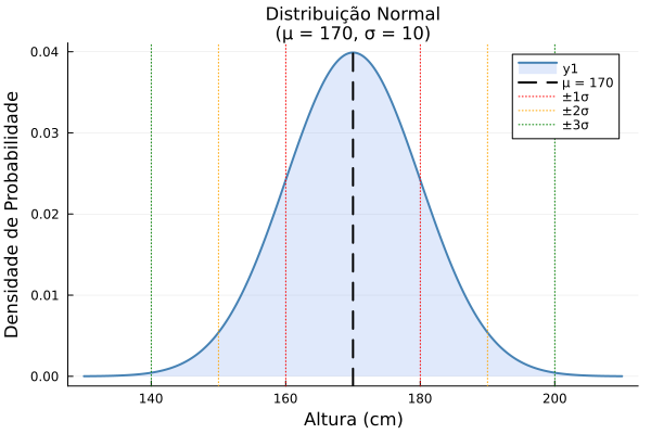
What is the normal distribution and why is it so important?
Few ideas in the history of science have proven as useful as the normal distribution. It shows up in the height of a population, in the measurement error of precision instruments, in financial asset returns, in the distribution of exam scores, in the average duration of industrial processes. It’s hard to name a field that doesn’t use it somewhere.
The reason isn’t magic — it’s mathematics. In its classical form, the Central Limit Theorem states that the mean of many independent, identically distributed random variables, each with finite mean and variance, tends to behave approximately like a normal distribution as the sample size grows. In other words, normality emerges naturally whenever many independent factors of the same nature combine — as long as each one has bounded variability.
A brief history
The bell curve has its origins in at least three thinkers spanning the 18th and 19th centuries.
Abraham de Moivre (1733) was the first to mathematically describe what we now call the normal distribution, while studying the approximation of the binomial distribution for large samples.
Pierre-Simon Laplace (1812) generalized and formalized the idea, making it central to probability theory and estimation methods.
Carl Friedrich Gauss (1809) used it to model observation errors in astronomical measurements, making the name Gaussian distribution synonymous with the curve. That’s why it carries his name, even though De Moivre and Laplace made equally essential earlier contributions.
Normal distribution formula
The probability density function (PDF) of the normal distribution is:
\[f(x) = \frac{1}{\sigma\sqrt{2\pi}} \, e^{-\frac{1}{2}\left(\frac{x - \mu}{\sigma}\right)^2}\]Each element of this equation plays a role:
| Symbol | Name | What it does |
|---|---|---|
| $\mu$ | Mean | Defines the center (peak) of the curve |
| $\sigma$ | Standard deviation | Controls the “spread”: larger $\sigma$, flatter curve |
| $\sigma^2$ | Variance | Squared measure of dispersion |
| $e$ | Base of the natural logarithm ($\approx 2.718$) | Creates the exponential decay |
| $\frac{1}{\sigma\sqrt{2\pi}}$ | Normalizing coefficient | Ensures the total area under the curve equals 1 |
We write $X \sim N(\mu, \sigma^2)$ to indicate that the variable $X$ follows a normal distribution with mean $\mu$ and variance $\sigma^2$.
What is the formula actually saying?
Despite its intimidating appearance, the formula has a simple visual logic:
- $\mu$ shifts the curve left or right, without changing its shape.
- $\sigma$ controls the spread: a larger standard deviation flattens and widens the curve; a smaller one makes it narrower and taller.
- The exponential term $e^{-\frac{1}{2}\left(\frac{x-\mu}{\sigma}\right)^2}$ makes the curve drop off quickly as $x$ moves away from the mean — the farther away, the closer the function’s value gets to zero.
- The coefficient $\frac{1}{\sigma\sqrt{2\pi}}$ is a scaling factor that doesn’t change the curve’s shape, it just ensures the total area under it is exactly 1 (as shown in the section on the Gaussian integral).
Fundamental properties
1. Symmetry
The curve is perfectly symmetric around the mean $\mu$. This implies that, for any value $c > 0$:
\[P(X \le \mu - c) = P(X \ge \mu + c)\]The left tail is an exact mirror image of the right tail.
2. Mean, median, and mode coincide
Because of the symmetry, the three measures of central tendency are equal:
\[\text{mean} = \text{median} = \text{mode} = \mu\]3. The total area is 1
Like any probability distribution for continuous variables, the integral of the PDF over the entire real line equals 1:
\[\int_{-\infty}^{+\infty} f(x)\, dx = 1\]4. The tails never touch the axis
The curve extends indefinitely in both directions, approaching the horizontal axis but never touching it. The normal density is positive for every real value, but that doesn’t mean the probability of observing exactly one specific value is positive. For continuous distributions, probabilities are computed for intervals, not isolated points: the probability that $X$ takes on exactly any single value is always zero. What this property actually says, then, is that no interval — however far from the mean — has strictly zero probability.
The Gaussian integral
Property 3 states that the total area under the normal curve is 1, but that isn’t obvious — the formula contains the expression $e^{-x^2}$, whose antiderivative doesn’t exist in terms of elementary functions. There’s no way to compute this integral the usual way, by finding an antiderivative and applying the Fundamental Theorem of Calculus.
The elegant workaround was discovered by Laplace and consists of computing the square of the integral using polar coordinates. Below is the full step-by-step calculation.
Step 1 — define the integral
Define:
\[I = \int_{-\infty}^{+\infty} e^{-x^2}\, dx\]The goal is to prove that $I = \sqrt{\pi}$. Since $e^{-x^2} > 0$ for all $x$, we know $I > 0$.
Step 2 — square it and turn it into a double integral
Since $I$ is a positive real number, we have:
\[I^2 = \left(\int_{-\infty}^{+\infty} e^{-x^2}\, dx\right)\left(\int_{-\infty}^{+\infty} e^{-y^2}\, dy\right)\]The two integrals have independent variables ($x$ and $y$), so they can be combined into a single double integral over the whole plane:
\[I^2 = \int_{-\infty}^{+\infty}\int_{-\infty}^{+\infty} e^{-(x^2 + y^2)}\, dx\, dy\]Step 3 — switch to polar coordinates
Substitute $x = r\cos\theta$, $y = r\sin\theta$, with $r \ge 0$ and $0 \le \theta < 2\pi$. The area element transforms as:
\[dx\, dy = r\, dr\, d\theta\]And the exponent becomes:
\[x^2 + y^2 = r^2\cos^2\theta + r^2\sin^2\theta = r^2\]The double integral becomes:
\[I^2 = \int_0^{2\pi}\int_0^{+\infty} e^{-r^2}\, r\, dr\, d\theta\]Step 4 — solve the inner integral in $r$
Compute $\displaystyle\int_0^{+\infty} r\, e^{-r^2}\, dr$ by substitution. Let $u = r^2$, so $du = 2r\, dr$, i.e., $r\, dr = \dfrac{du}{2}$. When $r = 0$, $u = 0$; when $r \to +\infty$, $u \to +\infty$:
\[\int_0^{+\infty} r\, e^{-r^2}\, dr = \int_0^{+\infty} e^{-u}\, \frac{du}{2} = \frac{1}{2}\left[-e^{-u}\right]_0^{+\infty}\] \[= \frac{1}{2}\left(\lim_{u \to +\infty}(-e^{-u}) - (-e^{0})\right) = \frac{1}{2}(0 + 1) = \frac{1}{2}\]Step 5 — solve the outer integral in $\theta$
The inner integral doesn’t depend on $\theta$, so:
\[I^2 = \int_0^{2\pi} \frac{1}{2}\, d\theta = \frac{1}{2} \cdot 2\pi = \pi\]Step 6 — conclude
Since $I > 0$:
\[I^2 = \pi \implies I = \sqrt{\pi}\]Therefore:
\[\int_{-\infty}^{+\infty} e^{-x^2}\, dx = \sqrt{\pi}\]Step 7 — prove that the area under the normal curve is 1
Now show that the coefficient $\dfrac{1}{\sigma\sqrt{2\pi}}$ in the normal distribution formula is exactly what guarantees a total area of 1. Start from the integral:
\[\int_{-\infty}^{+\infty} \frac{1}{\sigma\sqrt{2\pi}}\, e^{-\frac{1}{2}\left(\frac{x-\mu}{\sigma}\right)^2}\, dx\]Substitution 1: let $u = \dfrac{x - \mu}{\sigma}$, so $x = \mu + \sigma u$ and $dx = \sigma\, du$. The limits of integration stay the same ($-\infty$ to $+\infty$):
\[= \frac{1}{\sigma\sqrt{2\pi}} \int_{-\infty}^{+\infty} e^{-\frac{u^2}{2}}\, \sigma\, du = \frac{1}{\sqrt{2\pi}} \int_{-\infty}^{+\infty} e^{-\frac{u^2}{2}}\, du\]Substitution 2: let $t = \dfrac{u}{\sqrt{2}}$, so $u = \sqrt{2}\, t$ and $du = \sqrt{2}\, dt$:
\[= \frac{1}{\sqrt{2\pi}} \int_{-\infty}^{+\infty} e^{-t^2}\, \sqrt{2}\, dt = \frac{\sqrt{2}}{\sqrt{2\pi}} \int_{-\infty}^{+\infty} e^{-t^2}\, dt\]Applying the result from Step 6 ($\int_{-\infty}^{+\infty} e^{-t^2}\, dt = \sqrt{\pi}$):
\[= \frac{\sqrt{2}}{\sqrt{2\pi}} \cdot \sqrt{\pi} = \frac{\sqrt{2} \cdot \sqrt{\pi}}{\sqrt{2} \cdot \sqrt{\pi}} = 1\]This shows that the coefficient $\dfrac{1}{\sigma\sqrt{2\pi}}$ is not arbitrary — it’s the exact reciprocal of the value of the generalized Gaussian integral, and its sole purpose is to guarantee that the total area under the curve equals 1, a required condition for $f(x)$ to be a valid probability density function.
The 68–95–99.7 rule
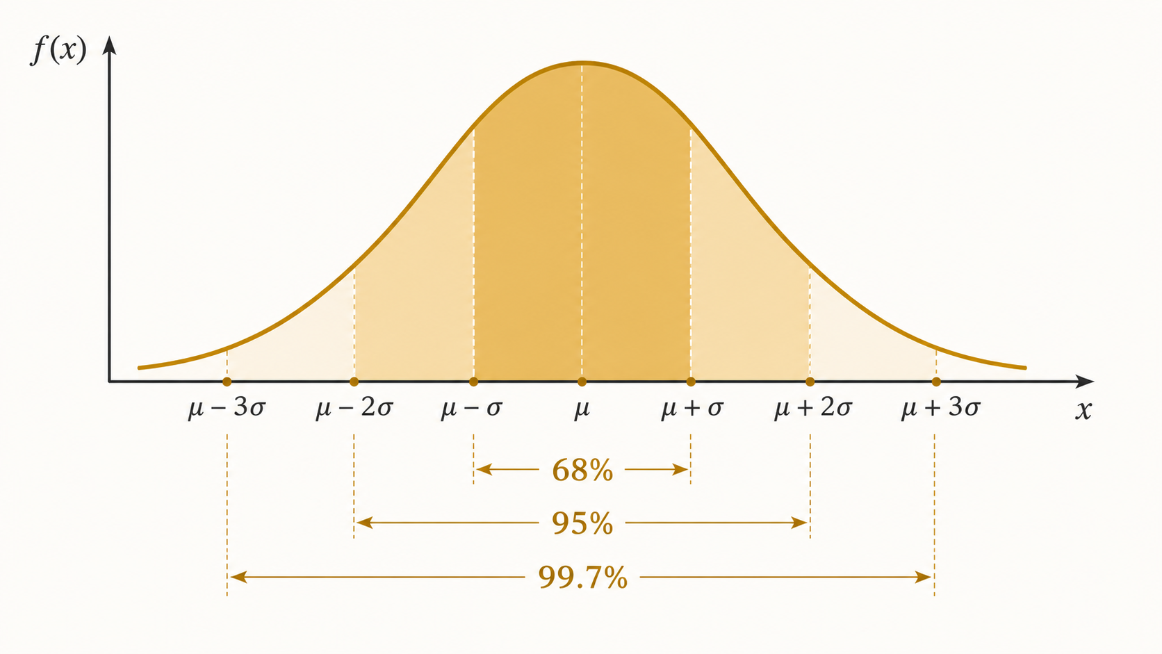
One of the most widely used properties of the normal distribution is the so-called empirical rule (or 68-95-99.7 rule). It describes how much probability is concentrated around the mean:
In plain terms:
- 68% of values fall within 1 standard deviation of the mean.
- 95% of values fall within 2 standard deviations of the mean.
- 99.7% of values fall within 3 standard deviations of the mean.
A value that falls beyond 3 standard deviations from the mean is rare — it happens in only about 0.3% of cases.
Careful
The 68–95–99.7 rule holds exactly for normal distributions. For data that's only "roughly bell-shaped" — especially with heavier tails than the normal predicts — the actual percentages can differ significantly. Use the rule with caution for skewed distributions or those with heavy tails.
How to calculate probability using the Z-score
When $\mu = 0$ and $\sigma = 1$, we get the standard normal distribution, denoted $Z \sim N(0, 1)$. Its PDF simplifies to:
\[\phi(z) = \frac{1}{\sqrt{2\pi}} \, e^{-\frac{z^2}{2}}\]Any variable $X \sim N(\mu, \sigma^2)$ can be standardized using the transformation:
\[Z = \frac{X - \mu}{\sigma}\]The resulting $Z$ value — the Z-score — tells you how many standard deviations the value $X$ is above or below the mean. This transformation matters because it lets you look up a single table (the Z table) to compute probabilities for any normal distribution, regardless of $\mu$ and $\sigma$.
How to use the normal distribution in practice
Before diving into examples, it helps to have the standard workflow clear:
- Identify $\mu$ and $\sigma$ from the problem statement.
- Convert the observed value to a Z-score using $Z = \dfrac{x - \mu}{\sigma}$.
- Look up the Z table to find $P(Z \le z)$.
- Use complements or differences of areas when you need probabilities for opposite tails or intervals.
- Interpret the result as an interval probability, never as the probability of a single exact point.
Worked examples of the normal distribution
Example 1: probability in a general normal distribution
Suppose a class’s grades follow $X \sim N(70, 100)$, meaning mean $\mu = 70$ and variance $\sigma^2 = 100$ (so $\sigma = 10$).
Question: what is the probability that a student scores less than 85?
Step 1: standardize the value $x = 85$:
\[Z = \frac{85 - 70}{10} = \frac{15}{10} = 1.5\]Step 2: look up the Z table for $z = 1.5$:
\[P(Z \le 1.5) \approx 0.9332\]Conclusion: there’s approximately a 93.32% chance a student scores less than 85.
Example 2: probability between two values
Using the same parameters ($\mu = 70$, $\sigma = 10$), what is the probability that a score falls between 60 and 80?
Step 1: standardize both bounds:
\[Z_1 = \frac{60 - 70}{10} = -1.0 \qquad Z_2 = \frac{80 - 70}{10} = 1.0\]Step 2: compute the probability between $-1$ and $1$ using the Z table:
\[P(-1 \le Z \le 1) = P(Z \le 1) - P(Z \le -1)\] \[= 0.8413 - 0.1587 = 0.6826\]Conclusion: there’s a 68.26% chance the score falls between 60 and 80 — exactly the $\pm 1\sigma$ interval predicted by the empirical rule.
Example 3: finding the value that corresponds to a probability
Still with $X \sim N(70, 100)$: what score $x$ is exceeded by only 10% of students? In other words, what is the 90th percentile?
Step 1: in the Z table, find the value $z$ such that $P(Z \le z) = 0.90$:
\[z \approx 1.28\]Step 2: undo the standardization to recover $x$:
\[x = \mu + z \cdot \sigma = 70 + 1.28 \cdot 10 = 70 + 12.8 = 82.8\]Conclusion: the 90th percentile of the distribution is 82.8. Only 10% of students score above 82.8.
When not to use the normal distribution
The normal distribution is powerful, but not universal. It’s not a good fit when:
- The data is skewed, like income or real estate prices — cases where the log-normal or exponential distribution may be more appropriate. Note that individual waiting times also tend to be skewed and are better modeled by distributions like exponential, gamma, or log-normal; averages of many waiting times, on the other hand, can approach normality thanks to the Central Limit Theorem.
- Values are restricted to an interval, like proportions between 0 and 1 — where the beta distribution is more natural.
- Rare count events are being modeled — where the Poisson distribution is more appropriate.
- Tails are heavy, as in extreme financial returns — where fatter-tailed distributions (like the Student’s t) better represent reality.
Recognizing when normality is a good approximation — and when it breaks down — is a central part of statistical work.
Next in the series
In the next post, we’ll explore the Poisson distribution, which models the count of rare events over a fixed interval of time or space — with a mathematical structure completely different from the normal, but with equally broad applications.
References
- De Moivre, Abraham. The Doctrine of Chances. 2nd ed. London, 1738.
- Laplace, Pierre-Simon. Théorie Analytique des Probabilités. Paris: Courcier, 1812.
- Gauss, Carl Friedrich. Theoria Motus Corporum Coelestium. Hamburg: Perthes & Besser, 1809.
- Casella, George; Berger, Roger L. Statistical Inference. 2nd ed. Duxbury Press, 2002.
- Stigler, Stephen M. The History of Statistics: The Measurement of Uncertainty before 1900. Harvard University Press, 1986.

Comentários