

Standard deviation is probably the most cited measure in reports, papers, and data presentations — and also one of the most misunderstood. Many people know it “measures dispersion,” but can’t really explain what that means, or why the formula has that square root in it.
This post settles that once and for all.
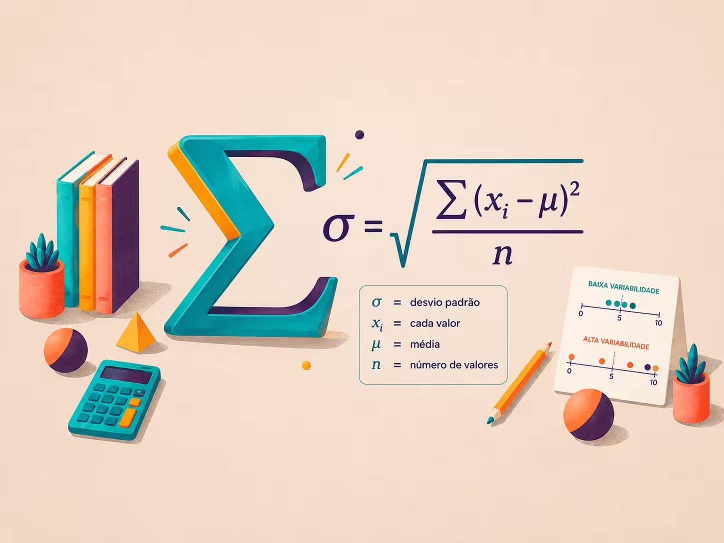
The problem standard deviation solves
Imagine two groups of students with the same average grade:
| Group | Grades | Mean |
|---|---|---|
| A | 70, 70, 70, 70, 70 | 70 |
| B | 40, 55, 70, 85, 100 | 70 |
The mean is identical, but the groups are completely different. In group A, everyone scored exactly 70. In group B, scores range from 40 to 100. Using only the mean to describe these groups would be misleading.
Standard deviation measures how far values spread out from the mean. More precisely, it’s the square root of the mean of the squared deviations — not the mean of the absolute distances (that measure exists too, and is called the mean absolute deviation). We’ll get to that distinction in the next section.
From the intuitive idea to the formula
The most direct idea would be to average the differences between each value and the mean. For group B above (mean = 70):
| Student | Grade (\(x_i\)) | Difference (\(x_i - \bar{x}\)) |
|---|---|---|
| 1 | 40 | −30 |
| 2 | 55 | −15 |
| 3 | 70 | 0 |
| 4 | 85 | +15 |
| 5 | 100 | +30 |
| Sum | 0 |
The problem: positive and negative differences always cancel out, and the sum is zero for any dataset. That’s not useful.
Solution 1 — use the absolute value:
\[\text{Mean absolute deviation} = \frac{1}{n}\sum_{i=1}^{n} |x_i - \bar{x}|\]This measure exists and has a name: it’s called the mean absolute deviation (MAD). It works, but the absolute value has inconvenient mathematical properties: it isn’t differentiable at zero, which makes it harder to use in optimization and more advanced statistical theory.
Solution 2 — square it:
Squaring also eliminates the signs, but uses standard algebraic operations. The result is the variance:
\[\sigma^2 = \frac{1}{n}\sum_{i=1}^{n} (x_i - \mu)^2\]The only cost is that variance is in squared units (for example, grades² instead of grades). To get back to the original unit, just take the square root — and that’s exactly the standard deviation.
The standard deviation formula
There are two versions, depending on the context.
Population standard deviation
Used when you have all the data for the group of interest (the entire population):
\[\sigma = \sqrt{\frac{1}{N}\sum_{i=1}^{N} (x_i - \mu)^2}\]Where:
- $N$ is the total number of elements in the population
- $\mu$ is the population mean
- $x_i$ is each individual value
Sample standard deviation
Used when you only have a sample and want to estimate the dispersion of the population:
\[s = \sqrt{\frac{1}{n-1}\sum_{i=1}^{n} (x_i - \bar{x})^2}\]Where:
- $n$ is the sample size
- $\bar{x}$ is the sample mean
The only difference is in the denominator: $N$ for the population version, and $n - 1$ for the sample version. The reason behind that difference — the famous $n - 1$ denominator — deserves its own explanation.
Why $n - 1$ and not $n$?
If you use $\bar{x}$ (the sample mean) in place of $\mu$ (the population mean), you’re already introducing a small error: $\bar{x}$ is computed from the very same data being used to measure dispersion. This creates a dependency that tends to underestimate the population’s true variability.
The exact mathematical correction is to divide by $n - 1$ instead of $n$. This adjustment is called Bessel’s correction, and it ensures that $s^2$ is an unbiased estimator of $\sigma^2$ — meaning that, on average (across many possible samples), the estimator gets the true value right.
Another way to think about it: when you compute $\bar{x}$, you “use up” 1 degree of freedom from the data. Of the $n$ values, only $n - 1$ can vary freely once the mean is fixed — the last value is determined by the others. That’s why you divide by $n - 1$, not by $n$.
Detail: $s^2$ is unbiased, but $s$ is not
The sample variance $s^2$ is an unbiased estimator of $\sigma^2$: $E(s^2) = \sigma^2$. The sample standard deviation $s$, however, is not exactly unbiased for $\sigma$: in general, $E(s) \neq \sigma$. This follows from the non-linearity of the square root (Jensen's inequality). In practice, for medium or large samples, the bias in $s$ is small and usually ignored.
When to use each version?
- $\sigma$ (population): when you have data for the entire population — for example, the grades of every student in a specific class you want to describe, with no intent to generalize.
- $s$ (sample): when you want to estimate the dispersion of a larger population from a sample — the much more common situation in practice.
Step-by-step calculation
Let’s calculate the sample standard deviation of group B’s grades: 40, 55, 70, 85, 100.
Step 1 — compute the sample mean $\bar{x}$:
\[\bar{x} = \frac{40 + 55 + 70 + 85 + 100}{5} = \frac{350}{5} = 70\]Step 2 — compute each squared deviation $(x_i - \bar{x})^2$:
| \(x_i\) | \(x_i - \bar{x}\) | \((x_i - \bar{x})^2\) |
|---|---|---|
| 40 | −30 | 900 |
| 55 | −15 | 225 |
| 70 | 0 | 0 |
| 85 | +15 | 225 |
| 100 | +30 | 900 |
| Sum | 2250 |
Step 3 — compute the sample variance $s^2$:
\[s^2 = \frac{2250}{5 - 1} = \frac{2250}{4} = 562.5\]Step 4 — take the square root:
\[s = \sqrt{562.5} \approx 23.72\]The square root isn’t just an algebraic detail: the variance $s^2 = 562.5$ is in points² — a unit with no direct interpretation in the context of grades. The square root brings the measure back to the original scale of the data, giving us points.
Interpretation: the standard deviation of group B’s grades is 23.72 points. Compare that to group A, where the standard deviation is zero — every grade equals the mean.
Standard deviation vs. variance: what’s the difference?
Variance and standard deviation measure the same thing, but on different scales:
| Variance (\(\sigma^2\) or \(s^2\)) | Standard deviation (\(\sigma\) or \(s\)) | |
|---|---|---|
| Unit | Original unit squared | Same unit as the data |
| Advantage | Convenient algebraic properties | Directly comparable to the data |
| Typical use | Theoretical calculations, ANOVA, regression | Reporting results, confidence intervals |
In practice, standard deviation is preferred for communication because it’s on the same scale as the data. Variance is used more internally, in mathematical derivations.
Important properties
1. Standard deviation is always non-negative
\[\sigma \ge 0 \qquad s \ge 0\]It equals zero only when every value is identical.
2. It isn’t robust to extreme values
A single value far from the mean can drastically inflate the standard deviation. For data with strong outliers, the interquartile range (IQR) is a more robust alternative.
3. Effect of linear transformations
If you transform the data with $Y = aX + b$, the standard deviation of $Y$ becomes:
\[\sigma_Y = |a| \cdot \sigma_X\]The shift $b$ (adding or subtracting a constant) doesn’t change the dispersion. The scale $a$ (multiplying by a constant) affects the standard deviation proportionally, without any squaring.
4. Sum of independent variables
If $X$ and $Y$ are independent random variables:
\[\text{Var}(X + Y) = \text{Var}(X) + \text{Var}(Y)\] \[\sigma_{X+Y} = \sqrt{\sigma_X^2 + \sigma_Y^2}\]Note that variances add up, not standard deviations. Adding standard deviations directly is a common mistake.
The coefficient of variation
Standard deviation has one limitation: its value depends on the scale of the data. A deviation of 5 kg when weighing elephants is negligible; the same 5 g deviation when weighing jewelry is enormous.
To compare dispersion across different scales, we use the coefficient of variation (CV):
\[CV = \frac{s}{\bar{x}} \times 100\%\]The CV expresses the standard deviation as a percentage of the mean, making it comparable across datasets with different units or orders of magnitude.
Practical reference (approximate):
| CV | Interpretation |
|---|---|
| Up to 15% | Low dispersion |
| 15% to 30% | Moderate dispersion |
| Above 30% | High dispersion |
Careful
The CV is only interpretable when the mean is positive and the data doesn't include zero or negative values. For temperature data in Celsius, for example, the CV can be misleading.
When the mean is close to zero, the CV can grow artificially and lose any practical meaning. When the mean is negative, the CV can come out negative, making comparisons between groups problematic. Only use the CV when the mean is well away from zero and positive.
Practical example: comparing two groups
A researcher measures the response time (in milliseconds) of two algorithms, each run 6 times:
- Algorithm A: 210, 215, 212, 208, 214, 211
- Algorithm B: 195, 230, 205, 240, 198, 232
Means:
\[\bar{x}_A = \frac{1270}{6} \approx 211.7 \text{ ms} \qquad \bar{x}_B = \frac{1300}{6} \approx 216.7 \text{ ms}\]Standard deviations (sample):
\[s_A \approx 2.7 \text{ ms} \qquad s_B \approx 19.4 \text{ ms}\]Coefficients of variation:
\[CV_A \approx 1.3\% \qquad CV_B \approx 9.0\%\]Algorithm A is slightly faster on average — a lower response time means higher speed — and far more consistent. Algorithm B shows a higher average response time and substantially greater variability: roughly seven times the standard deviation of A. The 5 ms difference in the mean might look small, but B’s instability (a deviation of nearly 20 ms) is often the deciding factor in latency-sensitive applications.
The connection to the normal distribution
When data follows a normal distribution, the standard deviation takes on a precise meaning thanks to the 68–95–99.7 rule:
\[P(\mu - \sigma \le X \le \mu + \sigma) \approx 68.27\%\] \[P(\mu - 2\sigma \le X \le \mu + 2\sigma) \approx 95.45\%\] \[P(\mu - 3\sigma \le X \le \mu + 3\sigma) \approx 99.73\%\]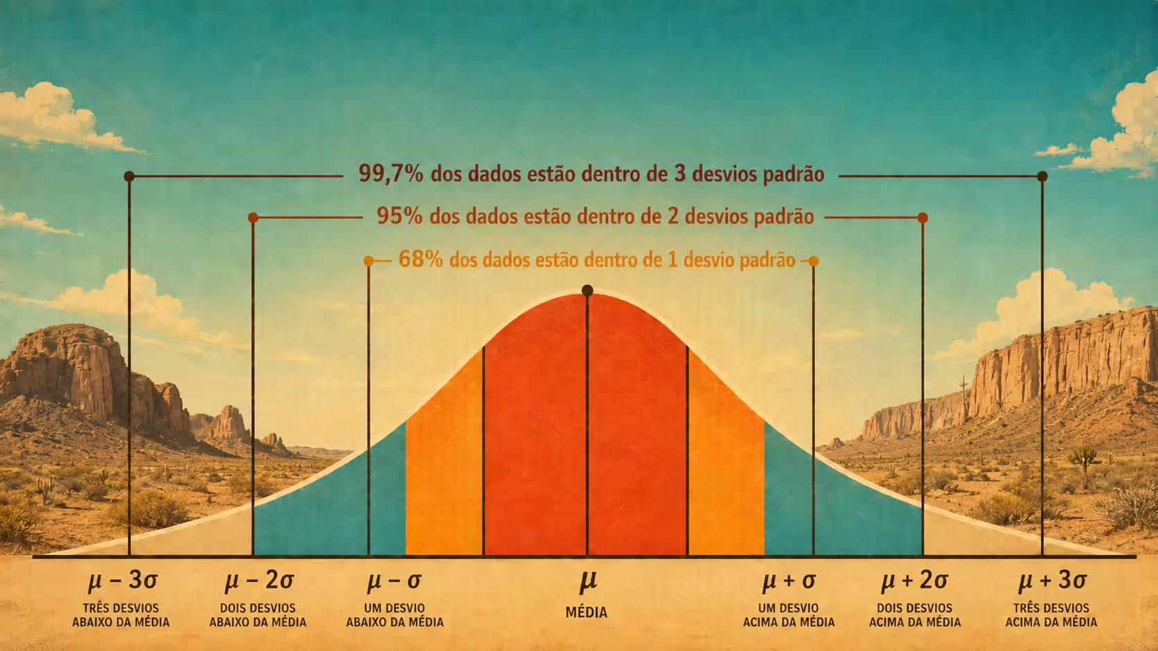
This means that, in a normal distribution, knowing the mean and the standard deviation is enough to fully describe the distribution — and to compute probabilities for any interval.
Outside of normality, Chebyshev’s theorem offers a weaker guarantee that still holds for any distribution: for any $k > 1$, at least $1 - 1/k^2$ of values lie within $k$ standard deviations of the mean.
The Z-score: standardizing with the standard deviation
Standard deviation is the natural unit for measuring “how far” an observation is from the mean. This idea is formalized in the Z-score (or standardized value):
\[z_i = \frac{x_i - \bar{x}}{s}\]The Z-score tells you how many standard deviations the observation $x_i$ is above (if positive) or below (if negative) the mean.
Example with group B’s data ($\bar{x} = 70$, $s \approx 23.72$):
The grade $x = 100$ corresponds to a score of:
\[z = \frac{100 - 70}{23.72} \approx 1.26\]The grade 100 is roughly 1.26 standard deviations above the mean. The grade $x = 40$, on the other hand:
\[z = \frac{40 - 70}{23.72} \approx -1.26\]The grade 40 is 1.26 standard deviations below the mean — symmetrically opposite the grade 100, as expected.
The Z-score is useful for:
- Comparing observations from different distributions — for example, a Math score and a Language score, which have different means and standard deviations.
- Spotting outliers — scores with z > 2 are uncommon in normal distributions (occurring in about 5% of cases); with z > 3, they’re rare (0.3%).
- Standardizing variables before scale-sensitive machine learning algorithms, such as regularized regression and k-NN.
When a variable follows a normal distribution, the Z-score lets you look up the Z table to compute interval probabilities — as covered in the post on the normal distribution.
Common mistakes
Confusing standard deviation with standard error. The standard deviation ($s$) describes the variability of individual data points. The standard error ($SE = s/\sqrt{n}$) describes the variability of the sample mean — it shrinks as sample size grows. These are different measures for different purposes.
Adding standard deviations. When summing independent random variables, variances add up ($\text{Var}(X + Y) = \text{Var}(X) + \text{Var}(Y)$), but standard deviations don’t add directly. To combine groups of data (for example, merging class A and class B into a single dataset), simply adding variances isn’t enough either — you also need to account for group sizes and the difference between their means. The variance of the combined dataset from two groups is:
\[s_{\text{comb}}^2 = \frac{(n_1 - 1)s_1^2 + (n_2 - 1)s_2^2 + n_1(\bar{x}_1 - \bar{x})^2 + n_2(\bar{x}_2 - \bar{x})^2}{n_1 + n_2 - 1}\]where $\bar{x}$ is the weighted mean of the two groups.
Using standard deviation for heavily skewed distributions. For strongly skewed distributions, like income or real estate prices, the mean and standard deviation can be poorly informative. Prefer the median and IQR in these cases.
Formula summary
| Measure | Formula | Use |
|---|---|---|
| Population variance | \(\sigma^2 = \dfrac{1}{N}\displaystyle\sum(x_i - \mu)^2\) | When you have the entire population |
| Sample variance | \(s^2 = \dfrac{1}{n-1}\displaystyle\sum(x_i - \bar{x})^2\) | When you have a sample |
| Population standard deviation | \(\sigma = \sqrt{\sigma^2}\) | Describing the population |
| Sample standard deviation | \(s = \sqrt{s^2}\) | Estimation and inference |
| Coefficient of variation | \(CV = \dfrac{s}{\bar{x}} \times 100\%\) | Comparing across different scales |
Worked exercise: heights of a class

Problem
In a class, the heights of six people were measured. After computing the group’s average height, it was found that each person deviates from the mean by a certain number of centimeters.
The absolute differences between each person’s height and the mean were:
\[|x_1 - \bar{x}| = 18 \text{ cm}, \quad |x_2 - \bar{x}| = 8 \text{ cm}, \quad |x_3 - \bar{x}| = 15 \text{ cm}\] \[|x_4 - \bar{x}| = 8 \text{ cm}, \quad |x_5 - \bar{x}| = 9 \text{ cm}, \quad |x_6 - \bar{x}| = 6 \text{ cm}\]Given that the standard deviation of these heights is approximately $11.5$ cm, interpret what this value means in the context of the figure.
Question: What does it mean to say the standard deviation of this group’s heights is about $11.5$ cm?
Solution
Step 1 — identify each person’s absolute deviation
| The absolute differences $ | x_i - \bar{x} | $ tell us, for each individual, how far above or below the mean their height is. Organized: |
| Person | \(|x_i - \bar{x}|\) (cm) | \((x_i - \bar{x})^2\) (cm²) |
|---|---|---|
| 1 | 18 | \(18^2 = 324\) |
| 2 | 8 | \(8^2 = 64\) |
| 3 | 15 | \(15^2 = 225\) |
| 4 | 8 | \(8^2 = 64\) |
| 5 | 9 | \(9^2 = 81\) |
| 6 | 6 | \(6^2 = 36\) |
| Sum | 64 | 794 |
Step 2 — compute the sum of squared deviations
\[\sum_{i=1}^{6}(x_i - \bar{x})^2 = 324 + 64 + 225 + 64 + 81 + 36 = 794 \text{ cm}^2\]Step 3 — compute the variance
Since we have the data for a specific group we only want to describe (not estimate a larger population), we use denominator $N = 6$:
\[\sigma^2 = \frac{\displaystyle\sum_{i=1}^{6}(x_i - \bar{x})^2}{N} = \frac{794}{6} \approx 132.33 \text{ cm}^2\]Step 4 — compute the standard deviation
\[\sigma = \sqrt{132.33} \approx 11.5 \text{ cm}\]This confirms the value given in the problem.
Step 5 — compare with the mean absolute deviation
To verify that standard deviation is not the same as the average absolute distance, let’s compute the mean absolute deviation (MAD):
\[\text{MAD} = \frac{|x_1 - \bar{x}| + |x_2 - \bar{x}| + \cdots + |x_6 - \bar{x}|}{6} = \frac{18 + 8 + 15 + 8 + 9 + 6}{6} = \frac{64}{6} \approx 10.67 \text{ cm}\]The MAD ($10.67$ cm) and the standard deviation ($11.5$ cm) are close, but different. Standard deviation squares the deviations before averaging — which makes larger deviations (like person 1’s 18 cm) weigh disproportionately more. That’s why $\sigma > \text{MAD}$ whenever the deviations aren’t all equal.
Answer
Saying the standard deviation of the heights is 11.5 cm means that, in terms of squared dispersion around the mean, each person in the group deviates from the average height by a magnitude equivalent to 11.5 cm. In other words:
- People with heights within the interval $[\bar{x} - 11.5\text{ cm},\; \bar{x} + 11.5\text{ cm}]$ are within one standard deviation of the mean.
- Looking at the figure: person 1 (18 cm deviation) and person 3 (15 cm deviation) fall outside that interval, while the rest (deviations of 8, 8, 9, and 6 cm) fall within it.
- The 11.5 cm standard deviation captures the group’s overall spread in a way that’s more sensitive to extreme values than the MAD (10.67 cm), since it penalizes those who deviate a lot from the mean more heavily.
Conclusion
The 11.5 cm standard deviation is not the simple average distance of heights from the mean (that would be the MAD = 10.67 cm). It's the square root of the mean of the squared deviations — a measure that gives more weight to people whose heights deviate more from the group's average.
Calculating it in practice: Julia code
using Statistics

data = [40, 55, 70, 85, 100]

data_mean       = mean(data)
sample_variance = var(data)       # denominator n − 1
sample_std      = std(data)       # denominator n − 1

println("Mean = ", data_mean)
println("Sample variance = ", sample_variance)
println("Sample standard deviation = ", round(sample_std, digits=2))
Expected output:
For the population version (denominator $N$):
n                    = length(data)
population_variance  = sum((data .- mean(data)).^2) / n
population_std       = sqrt(population_variance)

println("Population variance = ", population_variance)
println("Population standard deviation = ", round(population_std, digits=2))
Expected output:
Notice that the population variance ($450.0$) is smaller than the sample variance ($562.5$), since it divides by $N = 5$ instead of $n - 1 = 4$.
References
- Casella, George; Berger, Roger L. Statistical Inference. 2nd ed. Duxbury Press, 2002.
- Montgomery, Douglas C.; Runger, George C. Applied Statistics and Probability for Engineers. 6th ed. Wiley, 2014.
- Freedman, David; Pisani, Robert; Purves, Roger. Statistics. 4th ed. W. W. Norton & Company, 2007.
- Bessel, Friedrich Wilhelm. Untersuchungen über die Wahrscheinlichkeit der Beobachtungsfehler. 1838.

Comentários