
A Thousand People, a Hundred Thousand Voters: Where a Poll's Margin of Error Comes From
I redo by hand every calculation behind an election poll: why asking 1,000 out of 100,000 people works, where the three-point margin comes from, and why a 95% interval is right 94.98% of the time — not 95%. With the Julia simulation that confirms each number.
https://morrisonkuhlsen.com/polling-margin-of-error-sampling/
Every election the same scene plays out: a pollster interviews a thousand people, reports that a candidate stands at 38% “with a margin of error of three points”, and someone asks how a thousand people can say anything about a hundred million.
The short answer is that they can — and the size of the population barely enters the calculation. The long answer is about twenty formulas, and that is what this post does: it redoes by hand every number a poll reports, in a case where we know the true answer.
The trick to knowing it is to turn the problem around. Instead of starting from a poll and trying to guess the electorate, I make up the whole electorate and draw polls from it. Then you can ask things that are out of reach in real life: how many different polls could have come out? How many of them would be wrong?
The electorate I made up
There are $N = 100{,}000$ voters, distributed like this:
| Category | Voters | Share |
|---|---|---|
| Votes for A | 38,600 | 38.6% |
| Votes for B | 37,200 | 37.2% |
| Blank/spoiled | 3,600 | 3.6% |
| Abstains | 20,600 | 20.6% |
The parameter of interest is the share voting for A:
\[P = \frac{K}{N} = \frac{38{,}600}{100{,}000} = 0.386.\]A modelling choice that usually goes unnoticed: $P$ is the share of the electorate, not of valid votes. Those who abstain or spoil their ballot are in the denominator. Among valid votes it would be $38{,}600/(38{,}600+37{,}200) = 50.92\%$ — a very different number, answering a different question. It is worth checking which of the two the pollster reports.
The step that organizes everything that follows is to code the population as zeros and ones: $a_i = 1$ if voter $i$ votes for A, $0$ otherwise. Then
\[P = \frac{1}{N}\sum_{i=1}^{N} a_i = \bar{a},\]and estimating a proportion stops being a special problem — it is estimating a mean. All of sampling theory for means applies for free.
How many different polls could exist
The poll interviews $n = 1{,}000$ people by simple random sampling without replacement: every subset of size 1,000 has the same chance of being drawn. How many are there?
\[M = \binom{100{,}000}{1{,}000} \approx 1.7 \times 10^{2{,}430}.\]That number does not fit in any floating-point type — the computation is done in logarithms, with $\ln\Gamma$. For comparison, the observable universe has about $10^{80}$ atoms.
This unimaginable collection is what gives meaning to everything that follows. When an interval is said to “have 95% confidence”, the statement is about this population of $10^{2{,}430}$ possible polls, not about the poll in your hands.
The exact distribution
How many of the 1,000 respondents say A? Call that number $y$. Its distribution is hypergeometric:
\[P(y = k) = \frac{\binom{K}{k}\binom{N-K}{n-k}}{\binom{N}{n}}.\]The formula comes from pure counting. Since all $\binom{N}{n}$ samples are equally likely, $P(y = k)$ is the fraction of them with exactly $k$ voters for A. To build such a sample you choose $k$ of the $K = 38{,}600$ voters for A, which can be done in $\binom{K}{k}$ ways, and fill the rest with $n - k$ of the $N - K = 61{,}400$ others, in $\binom{N-K}{n-k}$ ways. Every choice from the first group pairs with any choice from the second, so the counts multiply. It is the same calculation as matching $k$ numbers in the Brazilian Lotofácil lottery (post in Portuguese), with voters in place of balls.
The most likely value is $y = 386$, exactly $nP$, and even that comes up in only 2.60% of polls. If the draw were with replacement, $y$ would be binomial and that probability would be 2.59%: with a 1% sampling fraction, picking someone twice is so rare that the two distributions nearly coincide.
The estimator is unbiased
The poll reports $\hat{P} = y/n$. The first thing to check is whether it errs systematically in one direction. It does not:
\[E[\hat{P}] = P.\]The proof fits in three lines using inclusion indicators: each voter has probability $\pi_i = n/N = 1\%$ of being interviewed, and the sum of the indicators gives back exactly $P$.
That 1% is the sampling fraction, and it will come back.
Where the margin of error comes from
The variance of the estimator is
\[\operatorname{Var}(\hat{P}) = \frac{N-n}{N-1}\cdot\frac{Pq}{n},\]with $q = 1-P$. The first factor is the finite population correction, and it is what answers the question at the start of the post. Here it is
\[\text{fpc} = \frac{99{,}000}{99{,}999} = 0.99001,\]that is, it shrinks the variance by 1%. Practically nothing. That is why the size of the population barely matters: interviewing a thousand people in an electorate of a hundred thousand gives almost exactly the same precision as interviewing a thousand in one of a hundred million. What counts is $n$, not $N$.
Doing the arithmetic:
\[\operatorname{SE}(\hat{P}) = \sqrt{0.99001 \times \frac{0.237004}{1{,}000}} = 0.015318 = 1.53\%.\]The standard error is the standard deviation of the estimator’s distribution over the possible samples. It is not the error of this poll — it is the typical scale of the procedure’s errors.
The margin of error is $t_{0.975}(999) \times \operatorname{SE}$, with $t_{0.975}(999) = 1.96234$:
\[1.96234 \times 0.015318 = 0.0301 = 3.01\text{ points}.\]The newspaper’s three points.
Except that no pollster publishes exactly this number, because nobody knows $P$. Each poll puts its own $\hat{P}$ in place of $P$ in the standard-error formula and therefore reports a slightly different margin. The poll in the next section, with $\hat{P} = 37.7\%$, reports $\pm 2.99$; at the edges of what is plausible here, from 35.7% to 41.6%, the margin goes from 2.96 to 3.04. It changes little because $\hat{P}(1 - \hat{P})$ is nearly flat near 50%.
The critical value $1.96234$ is that of the t distribution with 999 degrees of freedom (you can check it in the t table); with so many degrees of freedom it barely differs from the normal’s $1.96$. The site’s margin of error calculator uses $1.96$ and arrives at $\pm 3.00$, with the same exact coverage of 94.98% that appears further down.
A concrete poll
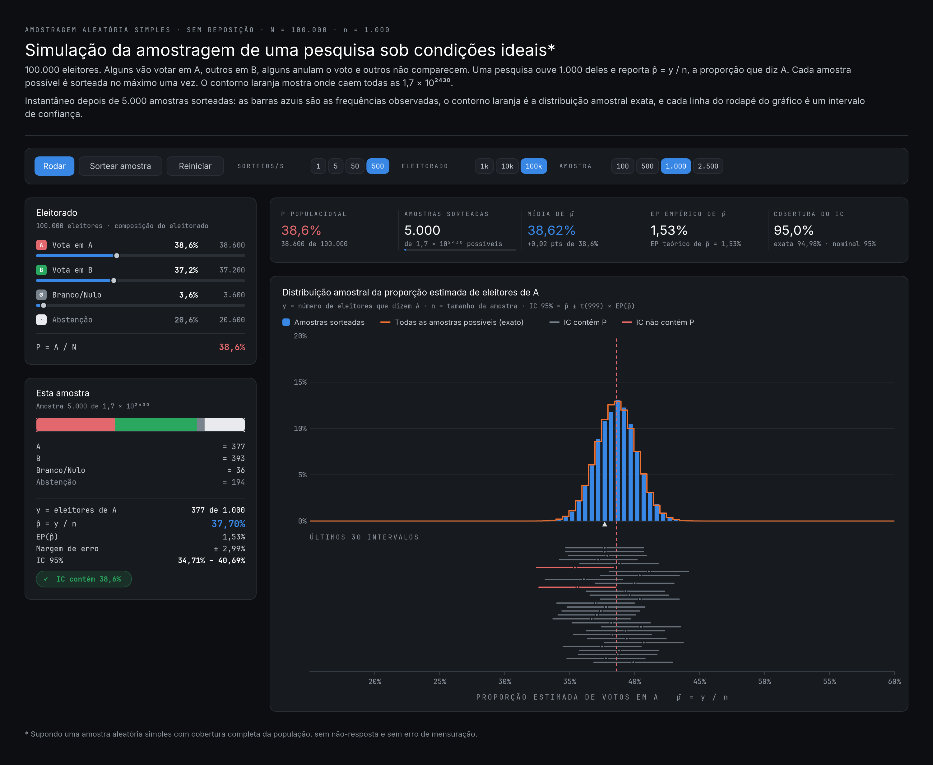
The last poll in the simulation interviewed 1,000 voters and found 377 saying A, that is $\hat{P} = 37.7\%$ against the true 38.6%. Its interval:
\[\text{CI}_{95\%} = [34.71\%,\ 40.69\%].\]And $P = 38.6\%$ is inside. This poll got it right.
What the interval does not mean: “there is a 95% probability that $P$ is between 34.71% and 40.69%”. $P = 0.386$ is a fixed number — either it is in the interval or it is not, and in this case it is, with probability 1. The 95% belongs to the procedure: of the $10^{2{,}430}$ possible samples, 95% produce an interval that captures $P$.
Except it is not 95%.
The exact coverage is 94.98%
This is the part that made me want to write the post. Since the population is known and finite, the exact coverage can be computed — add up the hypergeometric probability of every $y$ whose interval contains $P$. The result:
\[C = 94.9782\%.\]Not 95%. And the shortfall is neither an arithmetic error nor a lack of samples: it is a property of the procedure. Two causes, both checkable:
Discreteness. $y$ only takes integer values. The continuous coverage range went from 356.41 to 416.45; the discrete range goes from 357 to 416. A piece is lost at each end, and rounding has no reason to compensate.
The estimated standard error. The width of the interval is proportional to $\sqrt{\hat{P}(1-\hat{P})}$, which grows toward $\hat{P} = 0.5$. Since $P = 0.386 < 0.5$, samples that overestimate move toward 0.5, get wider intervals and cover more easily; those that underestimate produce narrower intervals and miss more often. Hence the lower tail (2.66%) is larger than the upper one (2.36%).
Two consequences worth saying out loud: running more polls does not fix it — coverage converges to 94.98%, not to 95%. And the effect is larger the smaller $n$ is.
The simulation confirms it
I drew 5,000 polls from this electorate, in Julia:
| Quantity | Observed | Theoretical |
|---|---|---|
| Mean of $\hat{P}$ | 38.6173% | 38.6000% |
| Standard error of $\hat{P}$ | 1.5266% | 1.5318% |
| Coverage of the 95% CI | 94.98% | 94.9782% |
That is 4,749 intervals that covered, against 251 that missed.
The observed bias of +0.017 point is 0.8 Monte Carlo standard errors from zero — consistent with the theoretical result. And the observed coverage tracks 94.98%, not 95%.
The core of the draw fits in a few lines. Shuffling the whole electorate and taking the first $n$ is a simple random sample without replacement:
using Distributions, Random, Statistics

N, n, K = 100_000, 1_000, 38_600
P = K / N
electorate = [fill(true, K); fill(false, N - K)]   # true = votes for A
fpc = (N - n) / (N - 1)
t = quantile(TDist(n - 1), 0.975)

function poll(rng)
    sample = shuffle(rng, electorate)[1:n]   # without replacement
    p̂ = mean(sample)
    margin = t * sqrt(fpc * p̂ * (1 - p̂) / n)
    (p̂, p̂ - margin <= P <= p̂ + margin)
end

rng = Xoshiro(2026)
res = [poll(rng) for _ in 1:5_000]
println("mean of p̂: ", mean(first.(res)))
println("coverage:   ", mean(last.(res)))
With this seed, coverage comes out at 94.7%. Another seed gives another number: with 5,000 polls, the Monte Carlo error of the coverage is about 0.3 point, which is why only the exact calculation can tell 94.98% apart from 95%.
The same experiment runs in the browser, in the poll simulator: you can draw the polls one at a time, change the sample size and watch the observed coverage approach the exact value.
What the margin of error does not measure
Everything above assumes simple random sampling with full coverage, no nonresponse and no measurement error. In practice:
- Complex designs (clusters, strata, weights) change the variance by a factor — the design effect — that usually lies between 1.5 and 3. A cluster sample of 1,000 may have the precision of 400 by simple random sampling.
- Nonresponse does not increase the variance: it introduces bias, which no increase in $n$ corrects. It is the error that does not show up in the margin.
- Measurement error — people who say one thing and vote another — is also bias, and also invisible to the margin.
The three-point margin measures only the variability of the draw. It is the smallest possible error, not the total error. When two polls from the same day disagree by much more than their margins would allow, the explanation is almost never in the draw.
The post can be summed up like this: the number the newspaper publishes is the easiest to compute and the least important of the errors. The three points come from a one-line formula, hold for any large electorate and, as the exact calculation showed, are not quite what they promise either. What decides whether a poll gets it right is who it managed to hear from, and no margin of error records that.
The simulation code is a Julia port of the dashboard by Raphael Nishimura.



Comments